
Introduction
During the last two decades, microscopy has been constantly trying to exploit new boundaries. By aiming for smaller details, cameras and other detectors needed to become more sensitive and less noisy due to less available photons per resolvable detail. Sensitivity was mostly improved by using higher light/laser power and increasing the quality of fluorescent markers; but the drawback of investing more light (or using short-wavelength with higher energy) is that, particularly when looking at living organisms, large amounts of phototoxic side products are created which degrade and eventually kill the organism. This makes it hard to say whether the observation is taking place at a healthy time point or at a decaying state.
One way to circumvent this problem came in 1990 with 2-photon laser scanning microscopy, which – back then – was meant to replace single-photon confocal microscopy (Denk et al., 1990). In principle, the use of near-infrared and infrared wavelengths could penetrate much deeper into a sample and was gentler to it (when compared with excitation using shorter wavelengths) as there was less phototoxicity. However, the cost was an almost prohibitively expensive Titanium-Sapphire laser which has only barely decreased in price today. Furthermore, as 2-photon laser scanning microscopy is a scanning technique, the acquisition is very slow – or if fast, very noisy. Large samples take hours to acquire and the only way to increase speed is to make smaller regions and restrict the field of view.
The new player is light sheet fluorescence microscopy, an illumination approach orthogonal to the detection that allows for a single plane illumination. This was first introduced by Richard Zsigmondy and Henry Siedentopf in 1903 using a slit-based system when they were working for Carl Zeiss. They called it the Ultramicroscope, and regrettably, it was soon forgotten.
It was reintroduced by Voie and colleagues in 1993 as a technique for orthogonal plane fluorescence sectioning (OPFOS), but the idea wasn’t really picked up by the scientific community until 2004 when Ernst Stelzer and colleagues refined the idea and built a new light sheet microscope called SPIM (Single Plane Illumination Microscopy). Both revivals used a cylindrical lens system to generate the light sheet improving its quality. They began by imaging embryonic development in animals and quickly adapted it to include the world of plants and nowadays even histopathology samples.
Technology In Brief
The main aim of light sheet microscopy is imaging a large sample with short time intervals under healthier conditions over longer periods (e.g. days) than compared to conventional types of microscopy or using the single plane illumination to improve single-molecule imaging (FCS, TIRF).
Looking closely at the illumination of a widefield microscope we notice that the sample which is placed in the plane of focus – where the energy of the excitation beam is the highest – is also excited above and below the focus (Fig.1A). The sample is moved to various planes of focus to acquire a z-stack and by this, the researcher obtains 3D information about the structures of interest and relation to secondary structures. If this was performed in a live cell experiment, planes above, in and below the focus would be exposed constantly which is detrimental to the sample. Aside from photobleaching, phototoxic side effects will cause the sample to be in non-physiological and later in apoptotic conditions, resulting in at least in extensive photodamage and even cell death.
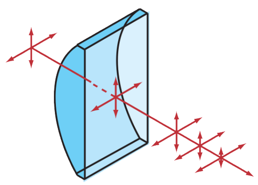
One could assume that using a point scanning device such as a confocal microscope would improve the situation as only individual points are excited. This is not the case because the beam, a) needs to be focused onto a certain point and thereby will also above and below the point of focus, and b) as the beam resides only briefly at each individual point, a much higher laser power is required which in turn causes even more damage to the sample (Fig. 1B/C).
One solution is to create a beam that is parallel to the focal plane (Fig. 1D). Above and below the plane of focus there is no excitation, and hence no additional negative effects in the out-of-focus planes. Rather than having a Gaussian beam profile, the beam is shaped by a cylindrical lens creating a sheet of light at and around the point of focus. The cylindrical lens maintains the round Gaussian beam’s profile in one dimension but compresses it in the other, as seen in Fig.2.
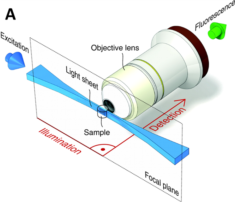
The light sheet allows the system to be designed in a way that only the sample plane in the focus of the imaging lens is illuminated. The emitted light is picked up by the imaging lens and detected by a camera. In terms of imaging, this has multiple benefits. Firstly, a single plane can be acquired in one quick snap due to multiplexing with the pixel array of the camera (benefit of the widefield system), and secondly, by illuminating one plane and avoiding exciting too much the planes above and below the imaging plane, the signal-to-background is improved (benefit of confocal in the z-axis). A light sheet diagram is shown in Fig.3.
In most light sheet systems, the majority of the optical components remain static while imaging. To obtain an image in 3D, the sample needs to be moved across the light sheet (other variations using adaptive optics sweep the sheet in XYZ across the sample). This is usually achieved by the movement of the sample holder which is a 3D- (XYZ) or 4D-stage (XYZθ, where θ is rotation). The movement in XYZ allows imaging of larger samples which can be larger than the already large FOV, which will require stitching in post-processing. The rotation gives access to the sample from multiple angles which can then be fused together. Because of this fusion process, the image will gain quality because the resolution will improve (see below for details).
Apart from that, there is a massive time benefit to be gained by this approach. Scanning a comparably sized sample on a confocal over minutes to hours can be reduced on a light sheet system to seconds and minutes. As mentioned before, phototoxic side effects are highly reduced by a factor of between 20-100x. And this is the main goal of light sheet microscopy: Image under physiological conditions for much longer and obtain more relevant data in live-cell experiments.
Light Sheet Optics
To obtain a sheet of light, a wide Gaussian beam needs to be converted to a sheet. When a beam is sent through a lens it will converge to the point of focus and diverge from there (Fig. 5). The numerical aperture (NA) is of special importance as it determines the strength of convergence and divergence, and thereby the usable field of view (FOV), as seen in Fig.4.
Two important distinctions need to be made regarding the depth of focus. If the NA of the imaging lens is very high it may be the determining factor for the depth of focus (in case the sheet is thicker than this). However, if the NA of the imaging lens is low the sheet is much thinner than the depth of focus and will thereby improve the signal to noise as only objects from within focus will be excited. Researchers in light sheet microscopy often strive to create the ‘thinnest’ or ‘ultrathin’ light sheet.
The simplest way to achieve a sheet of light is by introducing a cylindrical lens (very low NA) into the light path to create a 1D sheet. By focusing this pre-shaped beam onto the back-focal plane of the illumination objective, the sheet will be created at the focal point of this objective. The imaging objective is then placed perpendicular to the illumination objective and focused on the sheet.
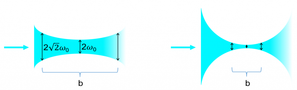
Theoretically – using a Gaussian beam, cylindrical lens and a high NA (1.4) illumination objective – a light sheet of thickness 0.24 µm is possible, but limited in usability as it would only have a depth of focus of 0.17 µm. On the other hand, a 10x/0.3NA water immersion lens would have a thickness of 1.1 µm with a depth of focus of 3.7 µm. Due to the nature of the system, this sheet will converge and diverge massively. Ernst Stelzer introduced a rule-of-thumb which is now well accepted in the field, which states that the usable width (b) of the sheet is maximal until it reaches twice the diameter of the waist (2ω0). By artificially lowering the NA it is possible to achieve a thicker sheet that remains parallel over a longer distance. This allows a larger field of view to be exposed. Typically, this can reach up to 1 mm in length and will have a thickness of 8 μm, at which point the imaging objective will potentially determine the depth of field and axial resolution.
New light sheet technologies often revolve around novel ways in which to generate a light sheet, including lattice light sheet and tiling light sheet, both discussed in their own application notes in our light sheet section.
Sample Preparation
Before researchers decide to perform light sheet microscopy, they should consider how to mount their sample in the most sensible way, because this will influence which light sheet configuration they will eventually have to use.
Live Samples
To enable live-cell imaging, samples must be immersed in some form of culture medium which requires objectives to be at least water dipping lenses. In order to retain the sample in its position, it has to be restrained. There are various options available, but it all comes down to the creativity of the researcher and the sample’s demands, as long as the mount is optically transparent, allows gas exchange (if necessary) and provides enough physical support to immobilize the living sample.
Initially, samples such as zebrafish were mounted by using a gel matrix, such as agarose (suitable due to its low-melting-point so as not to boil the sample) while mounting at a low enough concentration to not have a detrimental impact on the light sheet quality (Fig. 5A). As zebrafish do not tolerate temperatures above 32 °C for a long period of time, the agarose needs to be chilled down to below this temperature, which causes it to set quickly.
The sample can be otherwise mounted in a small volume/diameter syringe. The specimen is sucked in while being immersed in still liquid agarose. While the agarose is cooling down and sets, the sample can still be manipulated and optimally positioned. Once the agarose is set, the sample can be partially extruded into the water-filled sample chamber and is ready to be imaged.
Other ways of sample mounting have been developed such as the use of tubes made out of PTFE (Fig. 35C). This plastic has nearly the same refractive index as water and once immersed, is optically transparent and does not affect the light sheet properties. The tube approach has the additional benefit as one can use a small amount of potentially costly medium (few µl) that is separated from the rest of the sample chamber with its large volume (few ml).
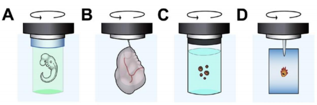
Plenty of different mounting techniques (Fig. 5A-D) have already been established and optimized for various sized samples, ranging from individual cells such as oocytes to entire organs such as brains.
Tissue Clearing
Light sheet microscopy is also a tool to image larger samples, which in comparison would take hours to image by conventional means. But large samples are quite opaque and light will be scattered and dispersed, for example, compartments rich in lipids can be imagined to function as microlenses. Depending on the tissue, pigments can also cause problems as pigments function as barriers and prevent light from ending up in the designated location.
To overcome those problems, tissue clearing was re-introduced (Fig. 6). Known for over a century, various methods using organic and inorganic solvents have been applied to larger samples (up to entire organisms such as mice) which enable researchers to look deeper into opaque structures and in more detail.
Some of those recipes will use organic solvents such as a mixture of benzyl alcohol and benzyl benzoate. Those solvents are very harsh and can easily destroy, or at least affect, various materials such as glues used on microscope lenses. A regular water dipping lens would suffer severely in the presence of those solvents. Hence, microscope companies have tried to overcome those issues as the clearing quality achieved by organic solvents is clearly superior to other methods using less harsh ingredients.
Drawbacks and Artifacts
Depending on the sample, light sheet microscopy enables the researcher to observe live processes never observed before. But unfortunately, it is not artifact-free.
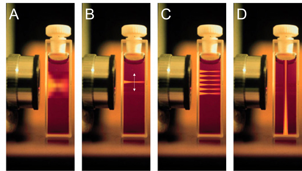
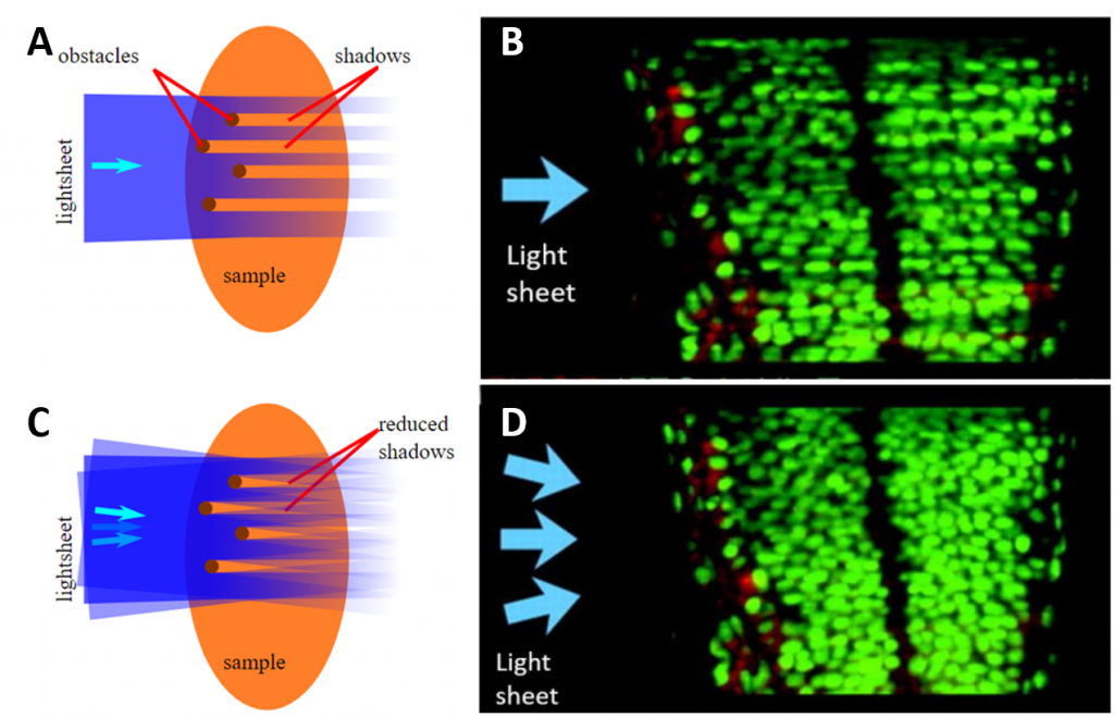
One of the biggest problems is striping patterns in the sample (Fig. 7A-B) – especially when using a standing wave and static mirrors. Those areas which seem to get less exposure are due to shadowing from optically dense structures and can be improved by pivoting the sheet (Fig. 7C-D). This problem can also be caused by dispersion which, due to the nature of the sample, may contain structures such as lipids which can act as microlenses in the tissue.
Another problem that leads to further non-uniformity of the sample illumination is the fact that the shape of the sheet and the intensity within will degrade as it passes through the sample. The same is true for emitted photons from deep within the sample not ending up in the imaging objective. Finally, sample mounting can be an issue. Researchers commonly state that light sheet microscopy is straightforward if not for the sample mounting.
Light Sheet Implementations
The standard light sheet implementation is SPIM, as seen in Fig.3, involving one microscope objective and one perpendicular light sheet. Due to the way this setup is shaped, it can also be referred to as L-SPIM (due to the sheet being 90° to the objective and making an L).
A great many other variations of SPIM exist, virtually one for every letter of the alphabet. Some of the main implementations of light sheet are discussed here, but be sure to check the other application notes for more advanced techniques on the light sheet learn page. Fig.8 shows some of the variations of SPIM.
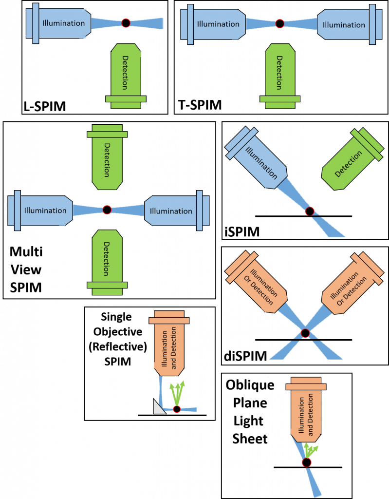
L-SPIM
The light sheet is created by using a cylindrical lens in conjunction with a large Gaussian beam. The pre-shaped (flattened) beam is focused onto the back focal plane of a lens, sent through it, and the sheet is created.
Using one sheet and one detection results in the L-SPIM layout (Fig. 3). With imaging depth, signal quality (excitation and emission) will degrade. In addition, L-SPIM uses a static sheet that only partially illuminates the sample. To overcome these issues, the sample has to be rotated, in the optimal case rotating four times by 90° and reassembled using sophisticated algorithms. This is computationally challenging in terms of speed and time. Furthermore, it will be quite prone to artifacts. Another solution is to have two light sheets, one from each direction.
T-SPIM
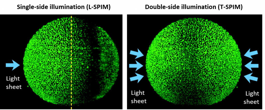
T-SPIM involves having two sheets from opposing sides which can be overlaid (Fig.8). As the intensity of a single sheet can decrease due to scatter and dispersion, the opposing sheet will increase imaging quality. Both sheets can be overlaid perfectly by matching their individual f. To increase the sheet and therefore image quality, researchers sometimes assign a slight offset to both as this will make the sheet more parallel over a longer distance. T-SPIM also results in less artifacts, as potential obstacles are illuminated from both sides, eliminating shadows, as seen in Fig.9.
In the T-SPIM layout, a large sample will be difficult to image, especially the rear, as the emitted light has to travel a long way into the sample and out of it. Dispersion and scattering will influence signals from deeper layers in the sample massively. To obtain a full stack of the sample only one rotation by 180° is required. More rotations at smaller intervals might improve the overall quality. As the FOV is required to be bigger individual file sizes will be larger, but fusion and the required computational processing can be quicker and easier. The T-SPIM layout can be used to illuminate very large samples on a macroscope at low magnification to get an entire organ for example imaged as quickly as possible. Various flavours are out there, which mainly differ in the number of sheets and their individual positioning, all aiming for a better imaging quality with fewer artifacts.
mSPIM
Multi-view spim (mSPIM or 4-lens SPIM) combines two excitation and two imaging light paths, where the cameras are synced with each other (Fig.8). For optimal resolution, the sample is imaged twice. First at 0° and a second time rotated by 45°. Objects imaged in XY can be resolved to a much higher detail compared to Z. This is owed to the way an object gets convolved by a series of lenses which is a function depending on the emission wavelength. The imaged object – be it infinitely small – will resemble a prolate spheroid, which is narrow (XY) and elongated (Z). This underlying convolution function is called the point spread function (PSF). When registering the stacks obtained at 0° and 45° – which requires fiducial markers around or in the sample – the PSFs from each individual point will be merged. Thereby, the resolution will become isotropic and improved by a factor of 3 in Z.
iSPIM and diSPIM
Inverted SPIM (iSPIM) and dual-view inverted SPIM (diSPIM) involve placing the objectives above the sample in a V-shape (Fig.8). The sample itself rests on some kind of platform. Either the objectives are moved up and down to acquire z-stacks or the sample is relative to the objectives. In essence, iSPIM is L-SPIM but at a different angle and with the sample fixed onto a stage. In diSPIM, excitation and emission occurs through both lenses. Excitation alternates between the two sides, as does the imaging. This system achieves isotropic resolution when used with two lenses of the same specifications. Sometimes this system can utilize different NA lenses. This will not result in isotropic resolution, but still dramatically improves the image quality.
Virtual Light Sheet
While the previous iterations of SPIM use a standing beam, some implementations of light sheet use a scanning beam.
By rapidly scanning a single beam and integrating the signal on camera, a virtual sheet can be produced. The beam itself needs to be of higher power compared to a standing sheet as each portion can only be excited for a fraction of the exposure time of the camera (which however is still much less compared to conventional widefield or confocal techniques). In this case, there is no requirement for a cylindrical lens.
This version of the light sheet allows a more sophisticated use of the camera. The position of the beam can be registered with the position of the row of pixels which is currently receiving a signal. All other neighboring rows are inactive and won’t detect a signal. As the Gaussian beam intensity drops off in all directions around the central axis, it will excite signal to a lesser extent all around the beam. With the single-row read-out, the out-of-focus signal can be rejected and the image will become crisper. This is also referred to as virtual slit mode.
Bessel Beams
Another variant of the scanning beam method was introduced by Eric Betzig’s lab. Rather than a beam with Gaussian characteristics, it is based on a Bessel beam which in theory is non-diffractive. In contrast to a Gaussian beam, it will propagate without diffraction and spreading. An important feature is its self-healing property. In case the beam gets partially obstructed at one point, it’ll reform further down the beam axis. Although this only happens in the ideal case, one can get a close to and by this achieve nearly no diffraction over a limited distance.
With the help of a lens called an axicon, a Gaussian beam can be converted into a Bessel-Gaus beam. Axisymmetric diffraction gratings or a narrow annular aperture placed in the far-field can achieve a similar outcome. The reason why it is tempting to use the Bessel beam – apart from its reduced sensitivity to diffraction – is that its profile is much smaller in diameter than the usually achievable Gaussian beam: <1μm. In essence, this allows super-resolution microscopy to be performed as the beam is now the limiting factor for resolving details, rather than the imaging lenses. Synchronization between beam position and the active line on the camera is crucial. For more on Bessel beams, please refer to our application note on lattice light sheet.
Data Storage and Processing
Fast data acquisition of large samples in 3D with very small pixels (high resolution) can result in a tremendous amount of data. Before one even starts to think about buying a light sheet system, considerations of proper data handling during imaging (no bottleneck between camera and PC to slow acquisition down) and post-processing should be done carefully. If a simple z-stack obtained in one color can already be hundreds of MB, imaging over time can easily reach 10-100 GB or more. Hence the appropriate hardware in the form of servers, SSDs, and fast data connections are required, and those will sometimes be even more expensive than the microscope itself.
Summary
Light sheet is a rapidly growing field in imaging due to its flexibility, low cost, and power as a platform. With the low phototoxicity, ability to image large samples and acquisition of images at a high speed, light sheet is the technique of choice for a number of researchers. The many flavors of SPIM allow for a customizable platform to be built in-house, for any imaging needs.
Download As PDF
References
Chen BC, Legant WR et al (2014) Lattice Light Sheet Microscopy: Imaging Molecules to Embryos at High Spatiotemporal Resolution. Science. 346(6208): 1257998. doi: 10.1126/science.1257998
Chung, K., Wallace, J., Kim, S. Y., Kalyanasundaram, S., Andalman, A. S., Davidson, T. J., Mirzabekov, J. J., , Zalocusky, K. A., Mattis, J., Denisin, A. K., Pak, S., Bernstein, H., Ramakrishnan, C., Grosenick, L., Gradinaru, V., & Deisseroth, K. (2013) Structural and molecular interrogation of intact biological systems. Nature. May 16;497(7449):332-7; doi: 10.1038/nature12107
Denk W, Strickler JH, Webb WW (1990) Two-Photon laser scanning fluorescence microscopy. Science. Apr 6;248(4951):73-6
Fahrbach FO, Voigt FF, Schmid B, Helmchen F, and Huisken J (2013) Rapid 3D light-sheet microscopy with a tuneable lens. Optics Express Vol. 21(18): 21010-21026. Doi: 10.1364/OE.21.021010
Huisken J, Swoger J et al. (2004) Optical sectioning deep inside live embryos by selective plane illumination microscopy. Science. Aug 13;305(5686):1007-9
Huisken, J. & Stainier, D. Y. R. (2009) Selective plane illumination microscopy techniques in developmental biology. Development. Jun;136(12):1963-75. doi: 10.1242/dev.022426
Kromm D, Thumberger T, Wittbrodt J. (2016) An eye on light-sheet microscopy, Methods Cell Bio. 133, 105-23
Krzic U, Gunther S et al. (2012) Multiview light-sheet microscope for rapid in toto imaging. Nat Methods. Jun 3;9(7):730-3. doi: 10.1038/nmeth.2064
Kumar A, Wu Y et al. (2016) Using Stage- and Slit-Scanning to Improve Contrast and Optical Sectioning in Dual-View Inverted Light Sheet Microscopy (diSPIM) Biol Bull. Aug; 231(1): 26–39. doi: 10.1086/689589
Lloyd-Lewis B, Davis FM et al. (2016) Imaging the mammary gland and mammary tumours in 3D: optical tissue clearing and immunofluorescence methods. Breast Cancer Res.Dec 13 18: 127. Dec 13. doi: 10.1186/s13058-016-0754-9
Pitrone PG, Schindelin J et al. (2013) OpenSPIM: an open-access light sheet microscopy platform. Nat. Methods. doi: 10.1038/nmeth.2507
Power, R. M. & Huisken, J. (2017) A guide to light-sheet fluorescence microscopy for multiscale imaging. Nature Methods. Mar 31;14(4):360-73; doi: 10.1038/nmeth.4224
Reynaud EG, Peychl J et al. (2015) Guide to light-sheet microscopy for adventurous biologists. Nat Methods. Jan;12(1):30-4. doi: 10.1038/nmeth.3222
Voie A. H., Burns, D. H., Spelman, F. A. (1993) Orthogonal-plane fluorescence optical sectioning: three-dimensional imaging of macroscopic biological specimens. J Microsc. Jun;170(Pt 3):229-36.
Weber M, Mickoleit M and Huisken J (2014) Light Sheet Microscopy. Methods in Cell Biology. Jan 01; 123:193-215; doi: 10.1016/B978-0-12-420138-5.00011-2
Wu Y, Ghitani A et al. (2011) Inverted selective plane illumination microscopy (iSPIM) enables coupled cell identity lineaging and neurodevelopmental imaging in Caenorhabditis elegans. Proc Natl Acad Sci U S A. Oct 25;108(43):17708-13. doi: 10.1073/pnas.1108494108