
Introduction
Fluorescence correlation spectroscopy (FCS) measures fluctuations in fluorescence intensity coming from any physical, chemical, or biological effects on the fluorophore of interest. In principle, light is focused in an area of the sample and the fluctuations in the fluorescence intensity in this area are measured. This fluctuation in fluorescence intensity can be caused by various dynamics, including the Brownian motion of particles. Brownian motion is the term for the random movement of molecules in a liquid/gas due to collisions with the other fast-moving particles in their environment. This results in random fluctuations in the position of a particle, in this case, a fluorescent particle or fluorophore.
FCS analysis on an area returns the average number of fluorophores in that area and their average diffusion time as they travel through the area. This data can be analyzed further to learn the fluorophore size, fluorophore concentration, solution viscosity, and diffusion coefficient. FCS is an extremely sensitive analytical tool as it is able to measure an incredibly small amount of molecules (nano/picomolar concentrations) within a small volume.
FCS Imaging System
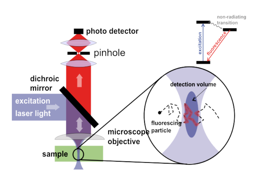
A typical FCS imaging system consists of a laser as an excitation source. The laser is focused on a specific area of the sample and the fluorescent molecules that cross the focal volume of the laser become excited and fluoresce. The emitted fluorescence goes back through the objective and is detected by a sensitive scientific camera, all seen in Fig.1. The data received is typically fluorescence intensity over time, but can be further analyzed with correlation analysis.
Correlation
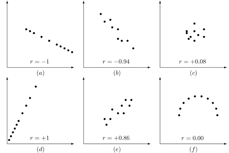
In order to see if two variables are related to each other, we can look at correlation. The relationship between two variables can be shown statistically which is referred to as the correlation coefficient (or Pearson correlation). Correlation coefficient values can range between -1 and +1 (noted as r), which are perfect negative/positive correlation respectively, and with 0 showing no correlation and no relationship between the two variables. Some example correlations can be seen in Fig.2.
Fluorescence Autocorrelation
Autocorrelation or serial correlation is the correlation between a signal and a delayed copy of itself. In other words, it is the correlation between two values from the same variable over successive time points. Unlike standard correlation, autocorrelation involves just one variable compared against itself, as opposed to comparing two variables against each other. This allows autocorrelation to represent the degree of the similarity between an original value and a value at a later time.
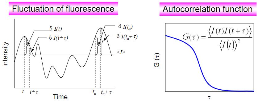
In FCS, fluorescence autocorrelation measures the fluorescence intensity at different time points, as displayed in Fig.3. This autocorrelation function (ACF) is an important variable when studying molecules, as the fluorophore diffusion coefficient (the average transition time of molecules within the laser observation volume) is inversely proportional to the ACF width, and the fluorophore concentration is inversely proportional to the ACF amplitude.
One of the common criteria that can be measured using FCS is the diffusion rate of the fluorescent molecules in and out of the observation volume. Once the fluorescent molecular enters the area, fluctuations in fluorescence intensity can be observed. By converting fluorescence fluctuations to an ACF, the diffusion coefficient and concentration can be extracted, as seen in Fig.4.

FCCS and FLCS
FCS has a number of daughter techniques, including fluorescence cross-correlation spectroscopy (FCCS) and fluorescence lifetime correlation spectroscopy (FLCS).
FCCS
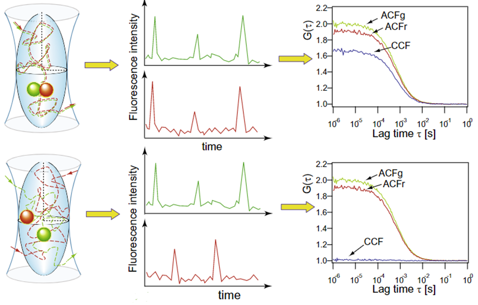
Fluorescence cross-correlation spectroscopy (FCCS) correlates signals from two different fluorophores, detected in two separate channels (green and red fluorescence, for example). When spectrally-different fluorophores are attached to two molecules, dual-color FCCS can be performed, showing the interactions between the two types of fluorophore. This is especially useful in order to study binding kinetics at low molecular concentrations. In essence, FCCS can be used to investigate the molecular binding partners and also the co-localization of two labeled proteins in a dynamic way, as seen in Fig.5.
To investigate if two labeled molecules A (green) and B (red) are binding partners, the ACF for each can be analyzed. If the fluorescence intensity over time of molecule A (ACFg) and B (ACFr) follow the same pattern and they are related, this would result in a high amplitude cross-correlation function (CCF) (Fig.5 upper panels). On the other hand, if the two molecules are moving around the defined volume independently of each other, the for these molecules will not be correlated resulting in low amplitude CCF (Fig.5 lower panels). Moreover, if only a subpopulation of particles has both labels (green and red), the amplitude of the CCF would lie between the two example cases, shown in Fig.5.
FLCS
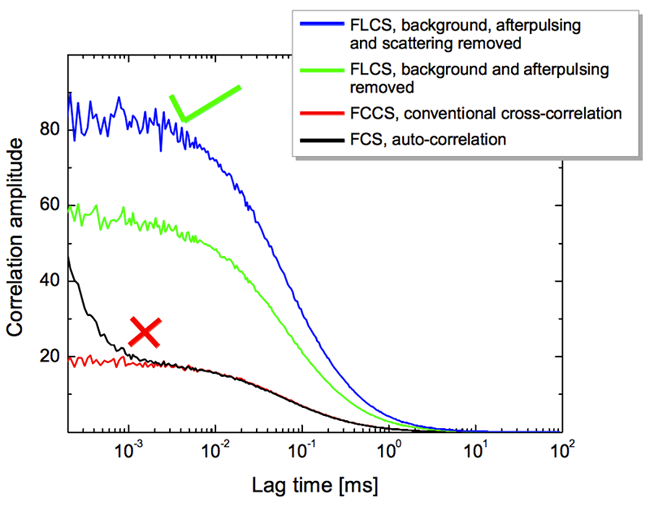
Fluorescence lifetime correlation spectroscopy (FLCS) uses pulsed lasers, rather than the continuous laser seen in FCS and FCCS. This allows for even more sophisticated analysis, with FLCS eliminating background or spectral crosstalk between fluorophores. This is useful when fluorophores cannot be separated, or when multiple fluorophores differ in their fluorescent lifetimes. A comparison of correlation amplitude between FCS, FCCS and FLCS can be seen in Fig.6.
FCS Applications
FCS can be coupled with several microscopy techniques such as confocal, two-photon, stimulated emission depletion microscopy (STED), and total internal reflection fluorescence (TIRF). These techniques involve focusing light on a sample, and by measuring the fluorescence intensity fluctuations with FCS, additional quantitative information can be obtained regarding fluorophore diffusion, fluorophore concentrations, and reaction rates.
For example, FCS has been widely used to elucidate the organization of lipids and proteins in cell membranes. This level of organization is crucial for cells as they play an important role in cellular processes such as endocytic and signaling pathways. By comparing the diffusion of several proteins, it has been shown that some proteins have more selectivity for certain domains. On the other hand, the increase in the diffusion coefficient upon cholesterol depletion represents the affinity of the concerned proteins for cholesterol-enriched domains. FCS is a powerful tool for studying molecular dynamics in living cells, providing quantitative answers on molecules and diffusion from within cells and cell compartments.
Cameras
As FCS is a technique that looks at a small number of molecules, the field of view (FOV) of a camera is an unimportant factor, with FCS detectors instead needing to focus on speed and sensitivity. A camera for FCS would need a high quantum efficiency and optimized pixel size, along with speeds up to 1000s of frames per second in order to detect fast dynamic binding events. New sCMOS camera technologies allow for high sensitivity and high-speed imaging of single-molecule events, making them suitable for FCS.
Summary
In FCS, excitation light is focused on a defined volume, once fluorescent molecules pass through this volume there are fluctuations in the fluorescence intensity. Accordingly, ACF curves can be obtained and important information can be achieved such as how fast molecules can diffuse in the plasma membrane, what concentrations of certain molecules are in solution, and locating binding partners in live cells.
When FCS was first introduced into the microscopy world around 50 years ago, it did not draw so much attention due to the drawback of having a low signal to noise ratio. However, recently after the incorporation of several microscopy methods together with the camera development, FCS has overcome this disadvantage and is transformed into a sensitive technique in several fields of study including biochemistry and biophysics. High frame rates and high sensitivity cameras (giving a higher signal to noise ratio) can contribute massively to the efficiency of the FCS method. Accordingly, back-illuminated sCMOS cameras will facilitate imaging with very low exposure time and therefore higher acquisition speed which is crucial for capturing the molecules at high speed. Very low noise performance is also important here.
References
Gerken, M., Krippner-Heidenreich, A., Steinert, S., Willi, S., Neugart, F., Zappe, A., Scheurich, P. (2010). Fluorescence correlation spectroscopy reveals topological segregation of the two tumor necrosis factor membrane receptors. Biochimica et Biophysica Acta (BBA) – Biomembranes, 1798(6), 1081–1089
Ghosh, A., Karedla, N., Thiele, J. C., Gregor, I., & Enderlein, J. (2018). Fluorescence lifetime correlation spectroscopy: Basics and applications. Methods, 140–141, 32–39
Hassler, K., Leutenegger, M., Rigler, P., Rao, R., Rigler, R., Gösch, M., & Lasser, T. (2005). Total internal reflection fluorescence correlation spectroscopy (TIR-FCS) with low background and high count-rate per molecule. Optics Express, 13(19), 7415
Ma, Y., & Ha, T. (2019). Fight against background noise in stimulated emission depletion nanoscopy. Physical Biology (accepted)
Macháň, R., & Wohland, T. (2014). Recent applications of fluorescence correlation spectroscopy in live systems. FEBS Letters, 588(19), 3571–3584
Nomura, Y. (2016). Fluorescence Correlation Analysis for Diagnosis Based on Molecular Dynamics. Biomedical Science and Engineering, Vol. 4, 2016, Pages 23-30, 4(1), 23–30
Tian, Y., Martinez, M. M., & Pappas, D. (2011). Fluorescence correlation spectroscopy: a review of biochemical and microfluidic applications. Applied Spectroscopy, 65(4), 115A-124A