
Introduction
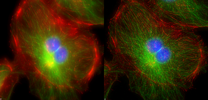
Microscopists and other scientists collect image data not necessarily for the value of the image itself, but for what it can them tell about the state of the sample. Unfortunately, the image data we collect is a combination of information given by the sample and distortion introduced by the imaging systems optical and detection properties. Furthermore, samples are often fairly three dimensional, and the collected two-dimensional image contains information both from the in-focus plane as well as out-of-focus regions of the sample. This can lead to an overall low signal to background ratio in the image due to the blurred signal from out of focus regions of the sample.
Several approaches have been created that minimize the contribution of out-of-focus parts of the sample to the final image. Confocal microscopy, for example, blocks out-of-focus light from reaching the detector and multiphoton illumination only excites signal in the focal plane itself. Another option is to mechanically slice the sample to a thinness equal to that of the lens focus depth, but this can only be used for fixed material embedded in a supporting matrix. However, none of these approaches address other aspects of the distortion introduced by an optical system such as aberration.
An image can be considered as a combination of information from the sample modified with the distortion inherent in the optical system. If the distorting effects of the system can be mathematically described, it should be possible to un-mix the hardware contribution to the image from the sample information. Deconvolution image processing aspires to do this, as illustrated in figure 1.
Taken from the Biology Imaging core website at Washington University at Saint Louis.
Common Uses Of Deconvolution
Deconvolution can be applied to any system as an approach to remove instrument effects from measured output in order to better represent the original signal. In microscopy, certain experimental needs favor the use of deconvolution.
In experiments where the goal is high-resolution volumetric data, and where every photon is precious, deconvolution is the common solution. As an example, tracking the 3D localization of a single labeled protein over time in an organism sensitive to illumination is exactly the type of experiment deconvolution excels at.
Point Spread Functions (PSFs)
When light from a fluorophore passes through the optics of a microscope, diffraction causes the light to spread. The signal captured from light originating from a single point (e.g. a single nanometer-scale fluorophore) will take on a characteristic shape known as a Point Spread Function (PSF). Figure 2 illustrates a model of the intensity profile of a point source imaged through a microscope in XZ, XY and YZ cross sections.
Every photon that is detected by a scientific camera has been spread in this characteristic way – mathematically, this is represented by the convolution of the ‘true’ image made up of the physical location of each point source and the PSF.
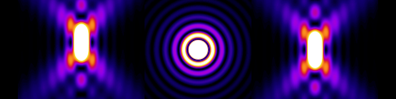
Taken from the website of the Biomedical Imaging Group, Ecole Polytechnique Federale de Lausanne and generated using the PSFgenerator software.
The spread of the PSF is given by the resolution of the optical system (which is typically at minimum around 200 nm in XY), this blurring represents the main barrier to resolving fine details in biological samples.
The PSF can be calculated if the wavelength of light and the numerical aperture of the optics are known. Otherwise, a practical measure of PSF of the microscope can be generated through optimal volumetric imaging of a small (below the diffraction limit) point source. This is commonly done with fluorescent beads less than 150 nm in size adhered to a substrate, a series of images sampled to Nyquist in XY and Z can provide a reasonably accurate description of the actual microscope system.
Practical measures of the PSF have benefits in that the PSF can be experimentally collected at differing locations to control for possible spherical aberrations. Similarly, if the sample to be deconvolved isn’t on a glass interface, locating the point source in a manner that better represents the sample to be deconvolved will increase the fidelity of the results.
The Logic Behind Deconvolution
By expressing the information provided by the sample as function (s) and the limitations inherent in the optical system as function (o), the convolution of these two functions is expressed as function (i):
i = s*o
The convolution, i, is the area under the curve of the product of the two functions as one is reversed and shifted against the other.
Doing this stepwise with functions consisting of large discrete arrays directly is computationally challenging. However, convolutions of functions in real space are equivalent to the multiplication of the Fourier Transforms of those functions, which can be displayed by the capital letters (I, S, O). Therefore, the convolution function i = s*o is equal to:
I = S x O
In Fourier space, deconvolution to isolate the sample information would be equivalent to:
S = I/O
The inverse Fourier Transform of I/O would, therefore, provide s, sample information with hardware contributions removed.
Unfortunately, this is made more complicated when working with measured data rather than functions because this requires the noise (n) inherent in our system to be addressed. Detector noise and the shot noise inherent in the photon signal itself complicate isolating s from i as the original function becomes:
i = (s*o) + n
Various algorithms take different approaches to deal with the inescapable noise contribution but the best way to ensure success is to start with high signal-to-noise images.
Software Implementation
There are many deconvolution algorithms that have been implemented in commercial or open-source software to deblur and or re-assign signal. Specific software packages will not be reviewed here, but the various mathematical approaches that are used will be briefly discussed. An excellent review of these approaches can be found in Sarder and Nehoral, 2005, from which the condensed summary below is extracted. For other insights, see the Molecular Expressions Microscopy section on Deconvolution Algorithms written by W. Wallace, L. Schaefer, J. Swedlow and D. Biggs.
Deblurring approaches aim to remove out-of-focus information from the image using low frequency information from the image plane and neighboring planes. They do this by blurring of the plane of interest or neighboring planes and subtracting the blur. The No Neighbor approach acts on the single plane in isolation, while nearest neighbor and multi-neighbor use planes above and below the focus plane. Deblurring commonly subtracts out low-frequency signal and does not reassign signal back to its origin. While this may provide more image contrast it also reduces total image intensity, making it less than ideal for quantitative imaging. These deblurring methods, which focus on removing low frequency information, are not good at removing noise.
Linear deconvolution methods incorporate information from all focal planes. Gaussian noise, such as found in CMOS cameras, is considered by some linear deconvolution methods. Inverse filtering, Wiener Filtering, Linear Least Squares and Tikhonov filtering use an experimentally derived PSF to un-mix sample from instrument blur. Here, the PSF is constrained to the experimentally derived or calculated form and only the image is iteratively changed. A workflow for common inverse filtering approaches is illustrated in Figure 3.
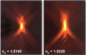
One consideration often ignored when using measured PSF in deconvolution is that both the image data and the PSF are discrete and intrinsically noisy measures of presumed continuous functions. As illustrated in Figure 4, noise and other subtle experimental issues can degrade the measure of the image or the PSF.
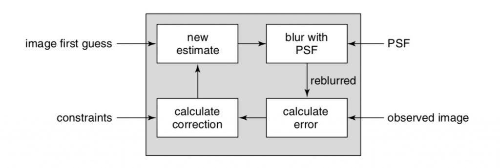
Image taken from (Biggs, 2010).
Weiner filtering, a linear deconvolution algorithm, considers gaussian noise from the detection hardware in its analysis. The frequency distribution of sample and hardware noise is incorporated to prevent high-frequency errors during the reconstruction. Similarly, Tikhonov filtering reduces the likelihood of high frequency solution with large noise contributions. These approaches do not extend the resultant frequencies beyond that found in the original PSF and can give negative intensity values in the deconvolved image.
Taken from the Olympus microscope primer webpage titled Introduction to Deconvolution.
Nonlinear Methods incorporate other details to address the problems associated with linear deconvolution algorithms. Constraints such as the solution can not contain negative values and expectations of the actual variability in the sample itself aid finding mathematical solutions with less error than the methods discussed above, at the expense of computation power. Janson Van Cittert, Non-linear Least squares, Iterative constrained Tikhonov-Miller deconvolution approaches are nonlinear methods that all assume that the all noise can be modeled as additive gaussian noise, but do not apply noise reduction in their process.
Statistical methods of deconvolving the sample from the image and hardware work well when the noise in the 3D data is large. Maximum Likelihood methods, and Maximum a Posteriori methods both can extend the resolution in the resulting image beyond that limited by the numerical aperture of the system. Maximum likelihood methods assume the noise is signal independent, accounting well for hardware noise but less well for Shot noise, which is related to signal. In contrast, Maximum a posteriori methods account for both gaussian hardware noise and Poisson distributed signal noise.
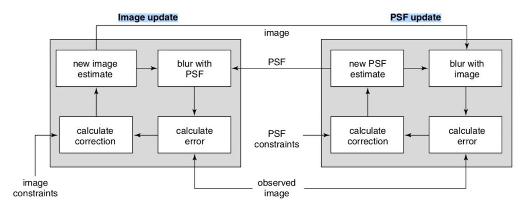
Blind deconvolution algorithms propose an initial PSF based on knowledge of the optics and sample, and then modify the PSF and image over many cycles while minimizing an error function. Over increasing numbers of cycles, the error is minimized as the calculated PSF better describes the system optics and the sample image is better isolated from the acquired image. Applying constraints, such as the result cannot be negative, or that the PSF must be symmetrical, aids selection of useful PSF models. A type of constrained iterative approach, blind deconvolution allow N iterations to be directed at improving the PSF, followed by N iterations directed at improving the image before repeating: PSF, image, PSF, image…. (Biggs, 2010). A workflow for blind deconvolution is illustrated in Figure 5. This approach can be quite computationally challenging.
Hardware And Image Collection Requirements
Optical imaging requirements
Deconvolution is a post-acquisition process and for good results, the initial image acquisition needs to have the best resolution and the highest signal to noise ratio possible. For samples located close to the glass interface, this often means high-NA low-aberration oil objectives and the best refractive index matching medium the sample will tolerate.
However, if the sample is immersed in a protein gel far away from the glass interface, lenses with lower NA but better index matching, such as glycerol or silicone oil immersion lenses may be more appropriate.
Selecting scientific cameras for optimal deconvolution reconstruction
The benefits of using deconvolution on light-sensitive samples or with a low total photon flux can be negated if the scientific camera isn’t efficient at converting photons to signal. Using high quantum efficiency cameras, such as back-illuminated devices, is one way to make every photon count. In addition, low readout noise and fast frame rates can allow for shorter exposure times and a shorter frame to frame delay.
The next consideration is sampling. To sample at Nyquist, measurement units need to be half as large as the resolution limit of the microscope, giving two measurements per optical resolution unit in XY and Z.
For a 1.4 NA lens detecting 500 nm light, the optical resolution limit laterally is 178 nm, and 775 nm axially. Nyquist sampling would then require a functional pixel size of 89 nm laterally and a focus step size of 388 nm. Given common camera pixel sizes of 4.25 µm, 6.5 µm and 11 µm, a 100x 1.4 NA lens used with cameras of those pixel sizes would provide measurements at either 42.5 nm, 65 nm, and 110 nm. Therefore, the best match would be the camera with the 6.5 µm pixel, giving a slight oversampling of the optical resolution.
Precisely controlled positioning in Z
Sampling optimally in Z is just as important as in XY. Z resolution as defined by Abbe is:
λ*2/NA^2
With the Nyquist criteria requiring sampling at a step size of ½ that or λ/NA^2.
Focus control can be carried out using a motorized lens or stage. For superior precision and speed between positions, though less overall range, piezo focus control accessories are commonly used.
Multi-focus imaging is a novel method that provides simultaneous acquisition of various sample focal planes on the camera chip. Integrating this approach, which is in active development (Hajj et al., 2017), could remove the time lag inherent in the serial collection of different Z positions.
Known Issues With Deconvolution
Image restoration by deconvolution is an exacting process. Some common experimental issues can render the processed result uninterpretable and must be addressed for successful restoration. Refractive index mismatch is a common issue, with significant problems occurring when the actual and input refractive indexes differ at the third decimal place as seen in Figure 4. The refractive index of glass varies with temperature (Waxler & Creek, 1973) so selecting the appropriate immersion oil with the appropriate refractive index for the temperature is common practice.
Also, the effective refractive index of the sample may differ depending on whether it’s attached to a glass surface or suspended in an aqueous media. Thicker and thinner areas of the sample may have effective differences in refractive index depending on whether the measurement volume is dominated by media, as in a thin region, or protein/lipid/carbohydrate as in the middle of a biological sample.
Many approaches also presume a relatively constant signal/noise ratio from the sample. Yet clearly some regions may have lower signal, and presumably lower signal/noise, than others. Thicker regions of the sample may have an issue with light scattering decreasing signal collection, also lowering the signal to noise ratio.
Summary
Deconvolution is a powerful analytical approach to gather as much information from a sample as possible. Success is dependent on using proper sample preparation, optimized optical and camera choices, and the appropriate analytical method. Proper application can increase the resolution and contrast of the resulting image.
References
Biggs, D. (2010) 3d Decovolution Microscopy. Curr Protoc Cytom. 2010 Apr; Chapter 12:Unit 12.19.1-20
Biology Imaging core website at Washington University at Saint Louis. (http://www.biology.wustl.edu/imaging-facility/specs-deltavision.php)
Biomedical Imaging Group, Ecole Polytechnique Federale de Lausanne website (http://bigwww.epfl.ch/algorithms/psfgenerator/)
Hajj, B., Oudjedi, L., Fiche, J-B., Dahan, M. & Nollmann, M. (2017) Highly efficient multicolor multifocus microscopy by optimal design of diffraction binary gratings. Scientific Reports. Volume 7, Article number: 5284
Olympus microscope primer webpage “Introduction to Deconvolution”. (https://www.olympus-lifescience.com/pt/microscope-resource/primer/digitalimaging/deconvolution/deconintro/)
Sage, D., Donati, L., Soulez, F., Fortun, D., Schmit, G., Seitz, A., Guiet, R., Vonesch, C. & Unser, M. (2017) DeconvolutionLab2: An open-source software for deconvolution microscopy. Methods. Feb 15;115:28-41. doi: 10.1016/j.ymeth.2016.12.015. Epub 2017 Jan 3.
Sarder, P., & Nehorai, A. (2006) Deconvolution Methods for 3-D Fluorescence Microscopy Images. IEEE Signal Processing Magazine, vol 32, p32-45
Wallace, W., Schaefer, L. , Swedlow, J. and Biggs, D. Algorithms for Deconvolution microscopy (https://micro.magnet.fsu.edu/primer/digitalimaging/deconvolution/deconalgorithms.html)
Waxler, R. M. & Creek, G. W. (1973) The Effect of Temperature and Pressure on the Refractive Index of Some Oxide Glasses. JOURNAL OF RESEARCH of the National Bureau of Standards – A. Physics and Chemistry. Vol. 77A, No. 6, p755