
Introduction
The digital image created by a scientific camera shows the level of light that falls on every pixel as an intensity value, this value is known as a gray level. With no light, the pixel is almost completely black, and when saturated the pixel is white. Everything in between is therefore a level of gray, hence a ‘gray level’. The bit-depth of the scientific camera is a representation of the maximum number of gray levels that the camera is capable of displaying. For example, an 8-bit camera is capable of displaying 256 gray levels, a 12-bit camera 4096 gray levels, and a 16-bit camera 65,535 gray levels.
Often, comparisons between the perceived brightness of biological features are made based on the gray level intensity values of the pixel. This can lead to potential misreporting of intensity values. When comparing images received from different cameras, either for comparison studies or when assessing new cameras for purchase, comparing the number of gray levels reported in a biological feature can lead to misleading comparison data or the purchase of incorrect scientific equipment.
There are various reasons why the intensity values reported from a sample can vary – the optical components used in the system, such as objectives and light sources, and different sample preparation methods can all affect the number of photons that are emitted by the sample and reach the camera. However, if all other variables are controlled for, the most influential element affecting the intensity values reported and the overall quality of the image is the camera.
Converting Photons To Gray Levels
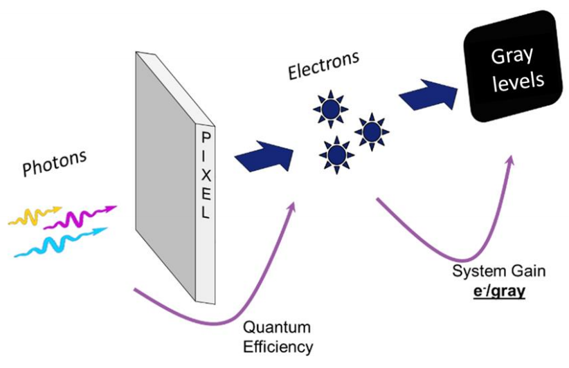
The creation of an image begins with the emission of photons from the sample. In many life science applications this involves focusing the emitted photons onto the camera sensor through the microscope. Photons hit the camera sensor, landing on the active pixels of the sensor array.
On the pixel, these photons are converted to photoelectrons – the ratio of conversion is dependent on the quantum efficiency (QE) of the camera sensor at the wavelength of the emitted photon. In theory, a 50% QE sensor would convert 100 photons into 50 electrons. Likewise, a 95% QE sensor would, in theory, convert 100 photons into 95 electrons.
Photoelectrons are then converted into a voltage which is converted into a digital signal – a gray level (Fig.1). The reported gray level intensity is a product of the conversion process that happens on the sensor. The conversion of electrons to gray levels is governed by the gain of the camera.
Gain values represent the number of gray levels that each photoelectron is converted to. The gain is represented as the number of electrons per gray level (e-/gray level). The lower the gain value is the more gray levels will be displayed per electron. For example, a camera with a gain of 1 would convert 1 electron to 1 gray level, whereas a camera with a gain of 0.25 would convert 1 electron to 4 gray levels (table below). This means that cameras with lower gain values are more sensitive changes in the signal, with a change in the electron number being represented by larger changes in the displayed gray levels.
| Gain (e-/gray level) | Gray Levels Per 1 Electron |
|---|---|
| 0.25 | 4 |
| 0.5 | 2 |
| 1 | 1 |
| 2 | 0.5 |
It should be noted that, when comparing intensity values, an image taken with a camera with a gain of 0.25 cannot be fairly compared to a camera with a gain of 1. Even if the detected electron signal is equal between both cameras, the gray level count of the camera with a gain of 0.25 will be four times higher than the camera with a gain of 1. The actual detected signal (in electrons) isn’t higher, just the gray level count. This becomes even more pronounced when using the EM-gain function of an EMCCD camera.
EM-gain Amplifies Gray Level Counts
Electron-multiplying charge-coupled device (EMCCD) cameras use an additional mechanism to multiply the number of photoelectrons generated from incident photons. Following photon to electron conversion, photoelectrons can undergo a process called impact ionization, often referred to as EM-gain, which amplifies the number of detected electrons. On modern EMCCDs this is a linear process where applying 10x EM-gain theoretically increases the electron count by 10x and 100x EM-gain increases the electron count by 100x. The goal of this process is to elevate the detected signal above the camera read noise threshold to improve the signal to noise ratio.
The amount of EM-gain used has a direct effect on the number of gray levels. As the number of electrons is amplified, so must the number of gray levels increase. For example, assume an EMCCD camera with a gain of 1 (1 electron = 1 gray level) detects 1 electron of signal and is amplified by 100x EM-gain. With this amount of EM-gain, the number of electrons increases from 1 to 100 which means that the number of gray levels also increases to 100. The signal level hasn’t changed, the original signal is still 1 electron. The difference is that this signal is now represented by 100 gray levels.
This can be problematic when making quantitative measurements as EM-gain can be changed dynamically by the user. If the user were to now increase the EM-gain to 300, using the previous example 1 electron of signal would now be displayed as 300 gray levels. If the two sets of data were then compared it would appear as though the second data set had more signal. It doesn’t, both data sets have 1 electron of signal, the difference is the increased EM-gain increasing the number of gray levels being used to display the data.
High EM-gain values mean low photoelectron counts are shown with more gray levels. Users collecting data using EM-gain must, therefore, be cautious to report data based on the unaltered signal. Using gray level values to compare the intensity of two images can result in misreporting the actual detected electron signal of the image.
Converting Gray Levels Back to Electrons
It is possible to calculate the photoelectron count of an image if certain camera parameters are known. These are the bias/offset and the gain.
Firstly, the camera’s background gray level value when no light is present must be identified – this is the bias/offset. With no light from any source reaching the camera sensor, the camera will display its lower limit gray level threshold. This threshold is used to protect data from the natural fluctuations of read noise, preventing signal values going below zero. The bias/offset should be removed before calculating the final signal level in electrons, for many Photometrics cameras this is typically 100 gray levels but this can be checked on the camera Certificate of Performance (CoP)
Next is the gain, camera gain can either be found on the Certificate of Performance (CoP) issued with every camera or it can be calculated experimentally, such as with the Photometrics Mean Variance Calculator.
A detailed explanation of how to record the bias of a camera and how to calculate the gain is found in the Photometrics Camera Test Protocol. Ultimately, the following equation can then be used:
Signal (e-) = (Signal in gray levels – Bias) * Gain
To determine the photoelectron count of a biological feature in the image, it is recommended to use a line profile to first determine its gray level intensity. This can be done by simply drawing a line over the feature using most commercial imaging software and measuring the peak signal level across the line. From the peak signal, subtract the calculated camera bias and multiply by the camera gain to calculate the signal in electrons.
Once an image has been converted back into photoelectrons, signal intensities of samples can be compared, either between different camera technologies or between different gain states on the same camera. Additionally, with calibrated samples or tightly monitored imaging parameters, the efficiency of photoelectron conversion can be used to measure camera performance.
Changing Camera Bitdepth
Higher bit-depths correlate to higher numbers of possible gray levels that can be recorded within the image. However, a common misunderstanding is that using higher bit-depths results in the collection of higher quality data. This leads some users to collect high bit-depth images even when the signal level is too low to make use of the full range of gray levels available. If a scientific camera supports the use of multiple bit-depths, lower bit-depths usually offer substantially increased speed. Users with low signal levels may be better off taking advantage of the high speed rather than the unnecessary high bit-depth.
It is important to note that cameras with multiple bit-depths often have different gain values associated with each bit-depth. This means that a 100 gray level signal at 16-bit may have not an equal number of detected electrons to a 100 gray level signal at 12-bit for example. It’s very important to have accurate bias and gain values of all bit-depths to be able to back-calculate to the real detected election signal. The tested gain values of each bit-depth are provided on the camera Certificate of Performance.
QuantView Reports Signal Directly In Electrons
In order to make converting an image back to electrons easier, a number of Photometrics cameras come with an advanced setting known as QuantView. This allows quantitative measurements to be easily taken, as turning on QuantView will instantly convert an image to electrons, without the need for any calculation steps.
Summary
Gray levels are used to construct the digital image produced by a scientific camera. However, due to differences in the way that photons are collected and processed, it is not possible to quantify fluorescence intensity without an understanding of the real electron signal level that the gray levels represent. Calculating the number of photoelectrons collected by each pixel in the image should be done to measure the true signal level of the sample or when comparing the performance of scientific cameras. If the bias and gain values are known, quantitative reporting of fluorophore intensity can be done, adding valuable quantitative data to existing visually-pleasing images.